Transformer-based deep learning for adaptive pedagogy under uncertain student preferences

This section describes how to dynamically categorize student preferences using SRE-TransformerNet. The strategy addresses tailored and inclusive education difficulties using modern methods. The training and assessment dataset includes varied student profiles and learning patterns. The hybrid SRE-TransformerNet architecture captures local and global student preference data dependencies using Swin-Transformer, ResNet, and EfficientNet modules. Novel preprocessing, feature selection, and data balancing strategies improve the model’s resilience and accuracy in complicated, high-dimensional data. In the succeeding sections, each framework component is detailed to illustrate how it enhances system performance. The proposed framework is shown in Fig. 1.

Table of Contents

Dataset description

The dataset used in this study was collected from multiple educational institutions across Manchester, UK, a diverse metropolitan region²⁶. It contains 202,000 records covering the years 2018 to 2024, offering a longitudinal perspective on student learning behaviors and outcomes. The data capture a wide range of information relevant to adaptive learning, including student preferences, academic habits, learning styles, course formats, engagement levels, and socio-demographic attributes. A detailed summary of these features is provided in Table 2. Data was collected from numerous schools and universities to reflect diverse socioeconomic origins, study settings, and academic specialties. Diversity increases the generalizability of results across educational environments. Institutional academic records, course evaluation forms, participation logs, and self-reported surveys provide objective performance measures and subjective learning preferences. For customized education and AI-driven adaptive learning, these insights allow models like SRE-TransformerNet to dynamically adjust pedagogical methods, assuring more inclusive and tailored learning experiences.

Table 2 Overview of dataset attributes.

Preprocessing steps

Several preprocessing procedures were used to guarantee high-quality input data for modeling²⁷. Before feeding the data into the model, missing values, outliers, feature selection, normalization, and data balancing were done. Category characteristics (e.g., study environment) were imputed using mode-based imputation, while numerical attributes (e.g., study hours) were imputed using median imputation to maintain dataset integrity. Using the interquartile range (IQR) approach, outliers were found and deleted to prevent model distortion. Adaptive Range Scaling (ARS) standardizes feature values while retaining dispersion in the initial transformation phase. This strategy preserves key data linkages and avoids scale differences from disproportionately affecting the model. Scaling is mathematically described in Equation (1):

$$\begin{aligned} Z’_{i} = \frac{Z_{i} – \mu _{Z}}{\sigma _{Z}} \times \delta _{Z} + \theta _{Z} \quad \forall i \in D \end{aligned}$$

(1)

The i-th sample’s scaled value is denoted as $Z’_{i}$, the original feature value is denoted as $Z_{i}$, and the mean and standard deviation of feature $Z$ are represented by $\mu _{Z}$ and $\sigma _{Z}$, respectively.Each feature is first standardized using two adaptive scaling parameters ($\kappa _A$ and $\mu _A$ in the preprocessing stage. Adjusting input variable ranges based on distributional characteristics reduces skewness and uniformly distributes dataset variation. This phase stabilizes the model and eliminates irregular magnitude bias. SFCWR is utilized next. Combine related qualities into one representation to save duplication and increase interpretability. Consolidation uses predictive feature power and correlations. Dynamic weights reflect component significance. The feature fusion step, shown in Equation 2, combines multiple original features into a single, more informative representation:

$$\begin{aligned} \Phi _{\text {combined}} = \sum _{r=1}^{\tau } \omega _r \cdot \phi _r, \quad \text {where } \sum _{r=1}^{\tau } \omega _r = 1 \end{aligned}$$

(2)

In this equation, $\Phi _{\text {combined}}$ is the new fused feature, $\phi _r$ denotes the r-th original feature, and $\omega _r$ is the adaptive weight assigned to it. The normalization condition $\sum _{r=1}^{\tau } \omega _r = 1$ ensures that the contributions of all features are kept in balance, so no single feature dominates the combination. This approach helps maintain overall consistency while producing a representation that is easier for the model to interpret and use effectively. The transformation controls recalibration as in Equation (3):

$$\begin{aligned} \Psi _{\text {adjusted}} = \Psi \cdot (1 + \alpha \cdot \zeta ), \quad \forall \Psi \in \mathscr {B} \end{aligned}$$

(3)

The transformed output is denoted as $\Psi _{\text {adjusted}}$ in this context, $\zeta$ measures the feature-related uncertainty, and $\alpha$ is a scaling coefficient that controls the transformation’s sensitivity. This set $\mathscr {B}$ contains all features undergoing recalibration. Adaptive scaling, targeted feature fusion, and uncertainty-aware transformation improve input data. These preprocessing strategies contribute to improved model robustness and precision, particularly in contexts involving complex or variable patterns, such as individualized learning behavior.

Data balancing

This work proposes Adaptive Data Balancing with Weight-Adjusted Sampling (ADB-WAS) to address the class imbalance in the dataset during data balancing. The model overfits the dominant class due to class imbalance, making it less accurate at classifying minority classes. ADB-WAS addresses this issue by weighting samples based on class frequency and feature relevance. Increased focus on underrepresented classes during model training²⁷.

Weighting each sample is the first step in the ADB-WAS procedure. This weight is inversely proportional to the sample’s class frequency, neutralizing class representation. The weight of the i-th sample, $\omega _i$, is computed using the Equation (4):

$$\begin{aligned} \omega _i = \frac{1}{g(D_i)} \cdot \sum _{j=1}^{q} \gamma _j \cdot H_{j,i} \quad \forall i \in S \end{aligned}$$

(4)

$\omega _i$ represents the sample’s weight for the i-th iteration, whereas $g(D_i)$ stands for the frequency of the class to which the sample belongs. The value of the j-th characteristic of the i-th sample is represented by the vector $H_{j,i}$, and its importance in classifying is indicated by $\gamma _j$. For this dataset, the ”q” stands for the overall count of features. In order to avoid bias against the majority class, this method gives minority training more priority with this weight adjustment. We resample the dataset using the weights that we acquired. Oversampling or maintaining higher-weight samples in the dataset is more common than undersampling lower-weight samples. In order to ensure that all classes are fairly represented during training, this resampling ensures that the dataset is balanced. By preserving the relationships between features and labels, the model is able to learn from any class.

The ADB-WAS approach balances the dataset while retaining feature correlations. The adaptive weight calculation prioritizes underrepresented classes during training while preserving feature distribution. This innovative strategy increases model generalization and classification accuracy, particularly for underrepresented classes. According to Equation 4, the weight-adjusted sampling strategy effectively balances the dataset, considering class distribution and feature relevance, leading to improved model performance.

Dynamic Feature Importance Selector (DFIS)

For feature selection, a new method called DFIS is introduced²⁸. This technique selects key dataset pieces while reducing superfluous or strongly associated attributes. The hybrid DFIS method retains just the most valuable characteristics for model training using statistical feature relevance assessment, dynamic correlation correction, and adaptive weighting. The Dynamic Feature significance Selector (DFIS) uses the Weighted Relevance Quotient to estimate feature significance. This statistic compares projected and actual outputs to each input attribute’s inherent variability to see how each affects model prediction accuracy. The WRQ score for the z-th feature is $\Omega _z$ and calculated as in Equation (5):

$$\begin{aligned} \Lambda _j = \frac{\sum _{i=1}^{M} \left| y_i – \hat{y}_i \right| }{\sum _{i=1}^{M} \left| f_{j,i} – \bar{f}_j \right| } \end{aligned}$$

(5)

In this expression, $y_i$ and $\hat{y}_i$ denote the actual and predicted target values for the i-th sample, respectively. The term $f_{j,i}$ corresponds to the value of the j-th feature for the same sample, while $\bar{f}_j$ is the mean of that feature across the dataset. The variable M represents the total number of samples. This formulation quantifies how much a particular feature contributes to reducing prediction error, thereby highlighting those features that carry stronger predictive signals relative to their internal variability. The second step of DFIS, called Dynamic Correlation Minimization (DCM), is designed to reduce redundancy by accounting for pairwise feature correlations. Features that exhibit high correlation with others add little new information and are therefore downweighted or removed. The correlation between the p-th and q-th features, denoted by $R_{pq}$, is computed as shown in Equation 6:

$$\begin{aligned} R_{pq} = \frac{\sum _{n=1}^{N} \left( X_{p,n} – \mu _{X_p} \right) \cdot \left( X_{q,n} – \mu _{X_q} \right) }{\sqrt{\sum _{n=1}^{N} \left( X_{p,n} – \mu _{X_p} \right) ^2 \cdot \sum _{n=1}^{N} \left( X_{q,n} – \mu _{X_q} \right) ^2}} \end{aligned}$$

(6)

Here, $R_{pq}$ is the correlation coefficient between features p and q, $X_{p,n}$ and $X_{q,n}$ are their values for the n-th observation, and $\mu _{X_p}$ and $\mu _{X_q}$ denote their respective means. If $R_{pq}$ exceeds a threshold $\theta$, one of the two features is removed to avoid duplication and multicollinearity. The third stage, Adaptive Relevance Adjustment (ARA), fine-tunes feature weights by combining relevance scores with correlation behavior. Features that are both highly relevant and less correlated with others are given larger weights. The weight assigned to the p-th feature, $W_p$, is calculated as in Equation 7:

$$\begin{aligned} W_x = \alpha \cdot R_x + (1 – \alpha ) \cdot \left( 1 – \left| \sum _{y=1}^{q} C_{xy} \right| \right) \end{aligned}$$

(7)

Each input variable in the suggested model has its own unique significance score, where $\Psi _k$ represents the weight given to the k-th feature. Features’ weight is determined by their relevance ($\Theta _k$) and interdependence with others ($\Lambda _{k,m}$), where m represents other dataset variables. A configurable hyperparameter $\delta$ controls the selection mechanism’s sensitivity, balancing relevance and redundancy. This adaptive method prioritizes variables with high predictive power and little overlap during selection. Adaptive Attribute Significance Evaluator (AASE) is a flexible, learning-aware tool for determining dataset’s most important characteristics. Instead of static filters, it uses three synergistic strategies: statistical relevance indicators to assess each attribute’s predictive contribution, actively diminishing the impact of high-correlation features, and weights that change with feature behavior and data context. This comprehensive selection technique emphasizes characteristics with relevant signals by suppressing noise and redundancy. AASE reduces overfitting and improves downstream model generalization by adjusting its internal logic to data form and distribution. Its adaptive core makes it suitable for real-world situations with dynamic, interdependent feature connections since it is compatible across domains, data kinds, and complexity levels.

Feature creation through Dynamic Feature Construction (DFC)

The Dynamic Feature Construction (DFC) strategy focuses on transforming raw features into more informative representations to better capture intricate dependencies and latent structures in the data^29,30. This transformation process enables the model to gain deeper insight into complex relationships that may not be immediately evident from the original features alone.

As an initial step, DFC generates what are referred to as Combined Influence Variables (CIVs), which reflect the interaction between two different features. These variables are particularly useful when the joint behavior of features offers more predictive value than the individual effects of each feature. For example, understanding how dedicated study periods interact with extracurricular involvement can reveal nuanced patterns in student success. Given two original input features $\chi _u$ and $\chi _v$, an interaction-based feature $\eta _{uv}$ is defined as in Equation (8):

$$\begin{aligned} \eta _{uv} = \chi _u \cdot \chi _v \quad \forall u \ne v \end{aligned}$$

(8)

By multiplying the values of $\chi _u$ and $\chi _v$, this equation yields $\eta _{uv}$, allowing the model to account for hidden synergistic effects between variables. After that, the approach calculates Relative Ratio Descriptors (RRDs) to measure the relative impact of one variable on another. These ratios may indicate priority allocation, such as between academic and recreational time. A ratio-based feature ($\zeta _r$) is computed using Equation (9):

$$\begin{aligned} \zeta _r = \frac{\chi _p}{\chi _q} \quad \text {where } \chi _q \ne 0 \end{aligned}$$

(9)

Here, $\chi _p$ and $\chi _q$ represent selected original features, and $\zeta _r$ encodes their proportional relationship. This ratio helps expose comparative trends that contribute to model interpretability and performance.

$$\begin{aligned} \theta _z = \frac{Z_z}{Z_w} \quad \forall z \ne w \end{aligned}$$

(10)

In Equation (10), $\theta _z$ represents the ratio of two characteristics $Z_z$ and $Z_w$, comparing them. This transformation reveals the significance of features compared to others.

Polynomial Features (PF) capture non-linear correlations between features, another crucial modification to DFC. Increase a feature’s power to account for fading or accelerating returns. Squaring Study Hours may show declining performance rewards as study time rises. The polynomial feature $\varsigma _x$ for feature $Z_x$ is computed as in Equation (11):

$$\begin{aligned} \varsigma _x = Z_x^2 \quad \forall x \end{aligned}$$

(11)

The polynomial feature $\varsigma _x$ is obtained by squaring the values of feature $Z_x$. To capture more intricate interactions, particularly when features and the target variable are non-linear, this transformation may be extended to cubic or quartic powers.

Summary Features (SF) aggregate information from related features. The Overall Engagement Score, which averages Study Hours, Extracurricular Activities, and Sleep Duration, shows a student’s overall involvement in numerous activities. The mean of a group of features is used to calculate the aggregate feature $\lambda _e$:

$$\begin{aligned} \lambda _e = \frac{1}{m} \sum _{k=1}^{m} Z_k \quad \forall k = 1, 2, \dots , m \end{aligned}$$

(12)

This Equation (12) uses $\lambda _e$ as the aggregate feature and $Z_k$ as the k-th feature in the averaged set. It aggregates data from numerous aspects to provide a more complete picture of the subject’s behavior.

Skewed features are transformed into regularly distributed features using Log-Transformed Features (LTF). Total Spending may be right-skewed; therefore, a logarithmic modification might stabilize its variance. The log-transformed feature $\nu _y$ is defined in Equation (13):

$$\begin{aligned} \nu _y = \log (Z_y + 1) \quad \forall y \end{aligned}$$

(13)

$\nu _y$ is the log-transformed feature generated from $Z_y$. The $+1$ guarantees the transformation works for zero-valued features. Skewed data is normalized, making it more similar to other characteristics and boosting model performance.

Dynamic Feature Construction (DFC) creates features that represent complicated data interactions, linkages, and non-linear patterns. Interaction variables, ratio features, polynomial features, summary features, and log-transformed features enrich the dataset. Newly synthesized characteristics help the model grasp data structure, increasing prediction performance. The equations utilized in this approach underpin each change, making the new characteristics understandable and mathematically sound.

Feature enhancement through Adaptive Data Mapping (ADM)

During feature enhancement using Adaptive Data Mapping (ADM)³¹, we refine features to improve predictive power and facilitate model learning of underlying patterns. ADM creates features that better describe data structure and adapt to feature attributes to improve model performance. The ADM approach adds innovative transformations depending on feature type.

ADM begins with Linear-Exponential Mapping (LEM), a transformation method that applies a linear or exponential mapping based on the feature distribution. The transformation of exponential or nonlinear characteristics is done using an exponential function, in contrast to the linear conversion of linear features. The feature $Z_t$ transformation is calculated in the following Equation (14):

$$\begin{aligned} T_t = \left\{ \begin{array}{ll} \alpha _t \cdot Z_t + \beta _t & \text {if linear relationship} \\ \exp (\gamma _t \cdot Z_t) & \text {if non-linear relationship} \end{array} \right. \end{aligned}$$

(14)

With $\alpha _t$ and $\beta _t$ regulating the linear transformation and $\gamma _t$ scaling the exponential transformation, the transformed value of feature $Z_t$ is represented by $T_t$ in this equation. This transformation adapts to feature distribution to capture simple and complex target relationships. Next, we rescale features by relevance and dataset hierarchy using Hierarchical Rescaling (HR). Composite and aggregate characteristics rescale differently than granular. Feature $X_p$ rescaling Equation (15):

$$\begin{aligned} S_p = \frac{X_p – \mu _{X_p}}{\sigma _{X_p}} \cdot \lambda _{X_p} \end{aligned}$$

(15)

The rescaled feature is denoted by $S_p$, the original value is denoted by $X_p$, and the mean and standard deviation are $\mu _{X_p}$ and $\sigma _{X_p}$ respectively. The scaling factor $\lambda _{X_p}$ addresses feature hierarchy, ensuring accurate scaling of key features in the dataset. Sequential Pattern-Aware Transformation is the third adaptive data modeling innovation. The method is intended to handle sequential or time-dependent characteristics. It allows the model to identify and adapt to long-term trends and patterns. Varying academic effort and results across numerous terms may indicate real advancement or regression that static characteristics may miss. The raw feature $\xi _r$, such study length or test performance, is dynamically changed to provide a temporally responsive characteristic $\mu _r$. Transformation definition:

$$\begin{aligned} \mu _r = \log (\xi _r + 1) \cdot \vartheta _r \quad \forall r \end{aligned}$$

(16)

The Equation (16) uses $\xi _r$ to represent the original sequential feature value, and $\mu _r$ to represent the modified feature that captures temporal dynamics. Add 1 to the log to maintain numerical stability and elegantly handle zero-input instances. To correct for changes in sensitivity or influence over time, the multiplier $\vartheta _r$ is used as a temporal adjustment coefficient. This change helps the model recognize changing behavioral patterns in consecutive data streams. The third ADM modification, Noise-Reduction Normalisation (NRN), smoothes features to minimize noise and outliers, particularly in high-variance data. This reduces extreme values by normalizing. Feature $W_r$ smoothing is shown by Equation (17):

$$\begin{aligned} W_r = \frac{1}{1 + \lambda _r} \cdot Z_r \end{aligned}$$

(17)

The smoothed feature is denoted by $W_r$, its original value is denoted by $Z_r$, and the degree of smoothing is controlled by $\lambda _r$. Stabilizing the model and reducing overfitting are achieved by adjusting noisy, high-variance features.

We create new or altered features that match data patterns using Feature Enhancement with Adaptive Data Mapping (ADM). Linear-exponential mapping, Hierarchical Rescaling, Sequential Sensitivity Adjustment, and Noise-Reduction Normalization enhance the dataset to provide the model with better inputs. Each transformation’s mathematical underpinnings guarantee that it improves model performance effectively and appropriately.

Classification with SRE-TransformerNet

The SRE-TransformerNet hybrid classification technique is presented in this study. It combines the designs of Swin-Transformer, ResNet, and EfficientNet in order to get the best possible performance on complex data sets^32,33, and³⁴. The goal of this approach is to effectively extract features while simultaneously capturing global and local interconnectedness through self-attention processes and deep residual linkages. For big datasets, SRE-TransformerNet is an effective solution because it provides excellent accuracy with little processing power. The flow of SRE-TransformerNet is illustrated in Algorithm 1, while Fig. 2 shows the layered architecture.

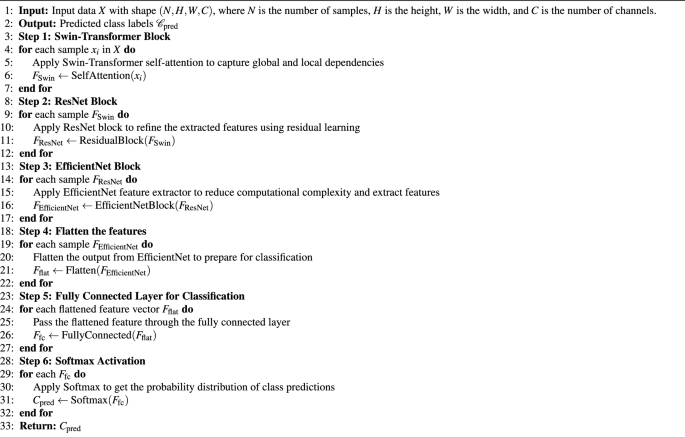
SRE-TransformerNet begins with the Swin-Transformer block, which is responsible for capturing spatial dependencies in the input feature map. By shifting non-overlapping windows across the data, the block applies self-attention to gather both fine-grained local details and broader global patterns. The attention mechanism for a feature map $\textbf{Z}$ is defined in Equation 18:

$$\begin{aligned} \textbf{H}(\textbf{Z}) = \text {Softmax}\left( \frac{\textbf{Z}_Q \cdot \textbf{Z}_K^\top }{\sqrt{d_q}} + \textbf{M} \right) \cdot \textbf{Z}_V \end{aligned}$$

(18)

Here, $\textbf{H}(\textbf{Z})$ represents the attention output. The matrices $\textbf{Z}_Q$, $\textbf{Z}_K$, and $\textbf{Z}_V$ correspond to the query, key, and value projections of the input, while $\textbf{M}$ is an added bias term. The scaling factor $d_q$ normalizes the dot product to stabilize training. The softmax operation ensures that the attention weights emphasize the most relevant regions, allowing the model to integrate both local and global contextual information. After the Swin-Transformer, the architecture incorporates ResNet blocks to deepen the model and strengthen feature representation. Residual connections are used here to combat the vanishing gradient problem, making it possible to train deeper networks more effectively. The ResNet block can be expressed as in Equation 19:

$$\begin{aligned} \textbf{Y} = \mathscr {G}(\textbf{Z}; \{\textbf{W}_j\}) + \textbf{Z} \end{aligned}$$

(19)

In this formulation, $\textbf{Y}$ is the block output, $\textbf{Z}$ is the input feature map, and $\mathscr {G}(\textbf{Z}; \{\textbf{W}_j\})$ denotes the transformation learned by the convolutional layers with weights $\{\textbf{W}_j\}$. By adding the input $\textbf{Z}$ back to the transformed features, the residual connection enables gradient flow through the network, improving convergence and supporting the learning of complex feature hierarchies. Finally, the EfficientNet block enhances feature extraction efficiency. This component uses compound scaling to balance network depth, width, and resolution, while depthwise separable convolutions reduce computational overhead. The block is defined mathematically in Equation 20:

$$\begin{aligned} \textbf{E}(\textbf{Z}) = \text {DepthwiseConv}\big (\text {PointwiseConv}(\textbf{Z})\big ) \end{aligned}$$

(20)

Here, $\textbf{E}(\textbf{Z})$ is the output of the EfficientNet block. Depthwise convolution processes each input channel independently, while pointwise convolution combines these results with a $1 \times 1$ operation. Together, they extract rich and discriminative features while keeping the number of parameters and computations low.

$$\begin{aligned} \mathscr {C}_\text {eff}(\mathscr {X}) = \text {DepthwiseConv}(\text {PointwiseConv}(\mathscr {X})) \end{aligned}$$

(21)

The EfficientNet block outputs $\textbf{F}_{\text {eff}}(\textbf{U})$, where $\textbf{U}$ is the input feature map. This block leverages two types of convolution operations: depthwise and pointwise. Depthwise convolution applies a separate filter to each individual input channel, drastically reducing the number of parameters. Pointwise convolution, implemented with a $1 \times 1$ kernel, then merges these channel-wise outputs to form a compact yet expressive representation. By combining these two operations, EfficientNet is able to extract rich features while keeping computational costs low, making it suitable for large-scale datasets.

Once the Swin-Transformer, ResNet, and EfficientNet modules complete feature extraction, their outputs are flattened and passed to a fully connected layer for classification. The probability distribution over the target classes is computed as shown in Equation 22:

$$\begin{aligned} \textbf{P} = \text {Softmax}\big (\textbf{W}_{\text {cls}} \cdot \textbf{h} + \textbf{b}_{\text {cls}}\big ) \end{aligned}$$

(22)

Here, $\textbf{P}$ denotes the predicted class probabilities, $\textbf{h}$ is the flattened feature vector from the previous layers, $\textbf{W}_{\text {cls}}$ is the weight matrix of the classification layer, and $\textbf{b}_{\text {cls}}$ is the corresponding bias term. The softmax function ensures that the outputs are normalized, producing a valid probability distribution across all classes. SRE-TransformerNet was chosen for experimentation because it integrates three complementary strengths: the Swin-Transformer’s ability to capture both local and global dependencies, ResNet’s residual learning for stable deep feature extraction, and EfficientNet’s lightweight yet powerful convolutional design. Together, these components create a robust and scalable framework that maintains accuracy while efficiently handling high-dimensional data, making it an excellent fit for diverse classification tasks.

Machine learning techniques like XGBoost excel at analyzing organized tabular datasets but struggle to grasp the hierarchical structures and temporal connections inherent in educational data. BERT-based models, which are designed for natural language processing, may not be ideal for learning preference categorization since they struggle to effectively analyze multimodal student behavioral data. The proposed learning framework, SRE-TransformerNet, combines a window-based transformer for fine-grained local dependencies, a residual learning stream for hierarchical consistency, and an optimised convolutional pipeline for scalable feature extraction. This integration provides precise context modelling and learning pattern adaptation, making the system ideal for personalised instruction. The hybrid model enhances classification accuracy and resilience by employing multi-scale attention mechanisms, skip connections, and computationally efficient operations on complex and high-dimensional datasets. The capacity to capture global trends and complex patterns balances performance in dynamic or imbalanced data. Its efficient architecture permits real-time decision-making, making it perfect for interactive, large-scale learning systems.

Interpretability and explainability in SRE-TransformerNet

Transparency, accountability, and very high performance are essential when using AI in educational contexts. Data analysis is essential for building trust, justice, and informed decision-making among educators, students, and other stakeholders. AI-generated outputs affect instructional planning, student assessments, and tailored learning routes, hence their logic must be clearly expressed and justified. The described learning architecture contains many interpretability levels. These levels clarify model logic. DFIS, or Dynamic Feature Importance Selector, prioritizes input variables based on their impact on model choices. With this information, educators may establish how learning styles, engagement, and socio-academic backgrounds impact student profiles and classification.

To further highlight the most important data segments, the model employs the visual encoding stream’s hierarchical attention mechanism. Graphically visualizing the areas that produce outcomes simplifies classifying learning types using this self-attention technique. The Contextual Sensitivity Score (CSS) ensures that individualised suggestions are based on student engagement and learning paths, not single indicators.

To boost model confidence, a rule-based decision-making framework explains learning modalities, instructional delivery tactics, and engagement analytics estimates. These structural aspects allow the model’s results to be understood and evaluated educationally. These interpretability techniques make the proposed system a trustworthy AI-driven helper for dynamic, inclusive, and student-focused learning environments by balancing technical correctness and ethical accountability.

link