


Traditional Chinese woodcut is a very interesting and diversified art, representative of abundant visual information with which the analysis may form certain indications of historical trends, cultural characteristics, and trends in artistic development. Still, classification and analysis require large amounts of human labor and are greatly subjective and easily mistaken. To handle the challenge, this section shows a completely automated approach with the use of machine learning techniques to classify Chinese woodcuts with high accuracy according to their artistic styles. First, this section describes how the dataset was collected, how contextual categorization is determined, and then presents the proposed strategy details for automating this process.
Data
This research utilizes a dataset including 900 high-quality photographs of traditional Chinese woodcuts, categorized into nine distinct artistic styles. Each style is regarded as a distinct category, encompassing 100 photographs that offer a thorough visual representation of this abundant artistic legacy. Equal number of instances for each category results in a balanced dataset. This dataset has been assembled from multiple web sources to guarantee extensive diversity and representation of diverse artistic genres. All images in the collection utilize the RGB color scheme, each exemplifying a distinct style of traditional Chinese woodcuts. The image dimensions in the dataset are inconsistent, requiring preprocessing to provide uniformity and compliance with machine learning models. All pictures have been downsized to a uniform dimension of 200 × 200 pixels to accomplish this objective. Furthermore, owing to the restricted sample size within each category, data augmentation methods such as random cropping, rotation, and flipping have been utilized to enhance data diversity and bolster the model’s generalization capacity. The identification of the artistic style for each sample has been conducted in conjunction with three art specialists. In this classification, each sample is initially segmented into three primary categories according to its origination time: (1) Early period (Tang to Ming dynasty), (2) Secondary period (Late Ming to Qing dynasty), and (3) Modern period (20th century and beyond). Each principal category is thereafter broken into three more specialized subcategories according to creative style. Each expert designates the target category for a sample, and the ultimate target category for each sample is established through majority voting. The agreement rate of 88.44% (perfect concordance on 796 out of 900 samples in the total dataset) signifies acceptable validity and precision of the categorization established by the experts. Figure 1 illustrates multiple instances of the photos contained inside this collection.
The samples in the dataset have been categorized based on the experts’ opinions into the following groups:
Early Period (Tang to Ming Dynasty):
-
1.
Religious: Most of them were Buddhist themes, featuring intricate patterns, bright colors, and often depicting deities and other mythical creatures.
-
2.
Literary: Images related to classic Chinese literature, such as novels and poetry, typically illustrating landscapes, historical figures, and allegorical scenes.
-
3.
Decorative: Decorative prints for home décor, including auspicious symbols, floral patterns, and geometric designs.
Secondary Period (Late Ming to Qing Dynasty):
-
4.
Nianhua (New Year Pictures): Colorful prints associated with Chinese New Year celebrations, often depicting gods of wealth, historical figures, and mythical creatures.
-
5.
Suzhou Prints: Delicate prints produced in the Suzhou region, known for their fine lines, soft colors, and intricate depictions of landscapes and figures.
-
6.
Yangliuqing Prints: Bright prints from the Yangliuqing region, in bold colors with dynamic composition, often presenting historical and mythological scenes.
Modern Period (20th Century and Beyond):
-
7.
Modern Woodcut Movement: Influenced by Western art and social realism, these woodcuts often convey social and political messages through imagery and intense symbolism.
-
8.
Revolutionary Woodcuts: Produced during the Chinese Revolution and the Cultural Revolution, these woodcuts frequently depict heroic figures, revolutionary scenes, and propaganda themes.
-
9.
Contemporary Woodcuts: A diverse range of styles that incorporate both traditional and modern elements, exploring a wide array of themes and techniques.

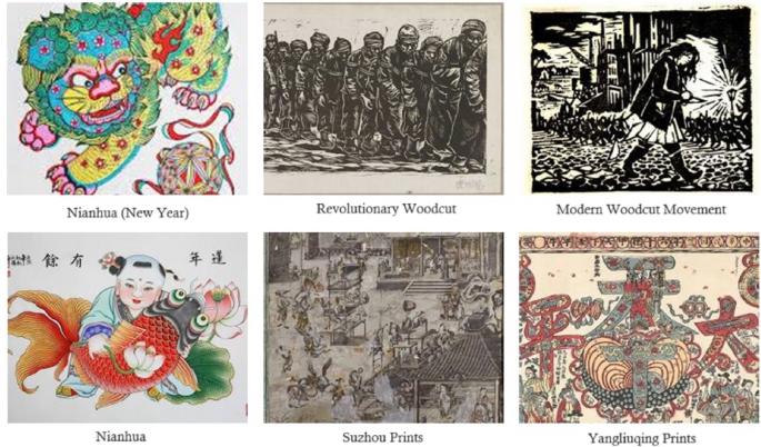
Some examples of images in the dataset.
The next section is dedicated to detailing the proposed model for the automatic classification of database samples based on the above categorization.
Proposed method
This section presents a cumulative learning-based strategy for the automatic classification of Chinese woodcuts based on their artistic styles. The proposed method aims to achieve a more accurate prediction system by combining the knowledge acquired from various deep learning models. Since the temporal information of the woodcut can be effective in narrowing down the categorization of its artistic styles, a CNN is employed to estimate the time period. Additionally, two separate CNN models analyze the image information to predict the artwork’s artistic style based on existing patterns. This combined model utilizes a meta-model based on decision trees and regression to ensemble the results from the three aforementioned models. The detection process in the proposed strategy can be summarized as follows (Fig. 2):
-
1.
Preprocessing of samples.
-
2.
Image analysis by CNN s to predict time period and artistic style.
-
3.
Ensemble of results using a meta-model based on decision trees and regression.

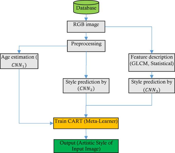
Diagram of the Proposed Approach for Artistic Style Classification.
The proposed method involves several steps, starting with the preprocessing of input images. According to Fig. 2, the preprocessing procedure consists of normalizing the dimension of the images and converting the color system of each sample into the RGB color model. This step is necessary in adapting the samples to image-processing models and eliminating redundant information. These preprocessed images are utilized simultaneously by three CNN models. First \(\:CN{N}_{1}\) in Fig. 2 is to predict the time period in which the artwork was created; each preprocessed sample would be classified into one of three categories: early period, secondary period, or modern period. Since the detailed categorization of artistic styles is based on temporal information, this data can play a significant role in achieving a more accurate detection model. Alongside this CNN model, two other CNN process the input sample (denoted as \(\:CN{N}_{2}\:\)and \(\:CN{N}_{3}\:\)in Fig. 2). \(\:CN{N}_{2}\), similar to \(\:CN{N}_{1}\), is a two-dimensional CNN that is fed by the preprocessed images, aiming to extract patterns related to the artistic style of each artwork based on the visual features present in the image. In contrast, \(\:CN{N}_{3}\:\)obtains its required input from a feature descriptor component. This one-dimensional CNN processes a set of statistical features and the Gray Level Co-occurrence Matrix (GLCM) of the image, rather than directly processing the images, and attempts to identify the artistic style of the artworks through a shorter set of image descriptor features. Each of the \(\:CN{N}_{2}\)and \(\:CN{N}_{3}\:\)models generates a predicted label for the artistic style variable. The predicted labels, along with the time period predicted by \(\:CN{N}_{1}\), are used as inputs for a decision tree and regression model CART. This CART model is trained based on the relationships between the predicted labels from the learning models and the target variable, allowing for a more efficient final output compared to conventional ensemble techniques.
Preprocessing
The database of images has varying dimensions, which makes it challenging to use them as inputs for machine learning models. Therefore, in the first step of the proposed method, the dimensions of all samples have been changed to 200 × 200 pixels to achieve a unified structure for introducing these samples to the machine learning models. All images were resized using bicubic interpolation. This method was chosen to maintain image quality during resizing without cropping, ensuring that the entire content of the woodcut is preserved. After resizing the samples, the preprocessing process targets the description of images in the color system. The initial images are described in RGB format, where the pixels of each sample are represented by intensity values for each of the three color layers in the range of [0, + 255]. Color features are significant in identifying the artistic style of the artworks; however, the intensity feature, which is visually represented as brightness, can be disregarded. To eliminate features related to intensity, the color system of each image is first converted from RGB to HSI. This action isolates the intensity feature in a separate layer from the image. Next, the I layer in the converted image is removed so that each image is described using the two layers H and S. Doing this results in each image being represented in a matrix format of 2 × 200 × 200. The resulting set forms the input for the learning models in the second phase of the proposed method.
Image analysis by CNNs for predicting the time period and artistic style of the artwork
In the process of identifying the artistic style of Chinese woodcuts, the stacked ensemble will use three CNN models to analyze the pre-processed images. The first CNN model will predict the time period, and the other two will attempt to identify the related artistic style category of the Chinese woodcut by processing the hidden patterns in the image. These three models have a similar architecture in layers, but the details of hyperparameter configuration are different among them. Figure 3 shows the structure of layer arrangement in these three CNN models.

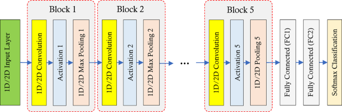
Layer Arrangement Structure in the CNN Models of the Proposed Stacked Ensemble.
The two CNN models, CNN1 and CNN2, are fed with preprocessed images; thus, their layer architectures are two-dimensional. On the other hand, CNN3 differs in input from the other two models. This CNN obtains its input data through statistical features and GLCM extracted from the initial image; consequently, its overall architecture is one-dimensional.
According to Fig. 3, all three CNN models used in the proposed stacked ensemble consist of 5 convolutional blocks. The first CNN model (for predicting the time period of the artwork) and the second CNN model (for predicting the artistic style of the artwork) accept HS layers with dimensions of 200 × 200 as input. The activation layers of these two models include a combination of LeakyReLU and ReLU functions in various blocks. Additionally, the pooling layers of these two networks use max and average functions. Considering the nature of the output of each model, the first CNN includes 3 neurons in its output layer (corresponding to the time periods), while the second CNN includes 9 neurons in this layer (corresponding to the artistic styles). In contrast, the third CNN feeds on 265 features described by the statistical properties and GLCM of the image, using a combination of sigmoid and ReLU functions in its activation layers. All pooling layers in this model are of the max type, and the final layer includes 9 neurons for determining the artistic style of the artwork. The configuration of each model has been conducted independently using a grid search strategy. In this process, various values for hyperparameters, including dimensions and the number of filters in the convolutional layers, the type of activation function, the type of pooling layer, and the size of the fully connected layer (FC1), have been examined. The search range for the filter dimensions of the convolutions has been established as a set, while the search range for the number of filters in each layer has been defined accordingly. Possible options for the activation function parameters in the activation layers have been considered as \(\:\left\{ReLU,LeakyReLU,Sigmoid\right\}\). Additionally, during the grid search process, different scenarios for using \(\:\left\{max,average,global\right\}\) functions in the pooling layers of the CNN models have been examined. The most suitable configurations obtained for each CNN model in the proposed stacked ensemble are presented in Table 1.
It is worth mentioning that during the grid search process, the training parameters for each model, including the \(\:\left\{SGDM,\:Adam\right\}\)optimization algorithm and minimum batch sizes of \(\:\left\{\text{16,32,64,128}\right\}\) were also examined. Based on the search results, the use of the Adam optimizer for CNN models 2 and 3 and SGDM for CNN1 yielded the best training performance. Additionally, the minimum batch size for all three CNN models was set to 32.
Cross-Entropy Loss was used for training all three CNN models (CNN1, CNN2, and CNN3), since it is designed for multi-class classification. Early stopping was used to avoid overfitting and make sure the training process did not run too long. If the validation loss remained the same for 10 consecutive epochs, training stopped. Training for 100 epochs gave the early stopping criterion the chance to decide when to end the training. For CNN2 and CNN3, which applied the Adam optimizer, the initial learning rate was 0.001, but for CNN1, which used SGDM, the learning rate was set to 0.01. The model used a step decay scheduler for learning rate, which cut the learning rate by 0.1 every 30 epochs. In addition, all CNNs had L2 weight decay with a factor of \(\:{10}^{-4}\) on their convolutional layers to help prevent overfitting. After the FC1 layers in every CNN, dropout layers with a rate of 0.3 were added. We chose a batch size of 32 because our experiments showed it gave the best balance between stable training, efficient use of resources, and the model’s performance, considering the type of data and model we were using.
As mentioned, the necessary input for model CNN3 is obtained through a feature descriptor component that extracts statistical properties and GLCM from the initial RGB image. It is important to note that this component extracts the mentioned features from the original RGB image. The continuation of this section is dedicated to explaining the process of preparing the necessary input data for model CNN3.
The first strategy employed for feature extraction from the initial images is the color correlation of pixels. To do this, the input image X in the RGB color system is mapped to 64 colors in the RGB space with dimensions of 4 × 4 × 4. This process is repeated using quantization for each pixel27.
$$\:{q}_{i,j}=\: \lceil N\times\:\frac{{p}_{i,j\:}}{{\text{m}\text{a}\text{x}}_{\text{p}}} \rceil$$
(1)
In the above equation, N represents the number of levels associated with the current layer, \(\:{p}_{i,j\:}\)denotes the pixel value at row i and column j in the current layer, and \(\:{\text{m}\text{a}\text{x}}_{\text{p}}\:\)refers to the maximum value corresponding to this layer. The quantized matrix is considered as the image X’ with a limited color space.
In the image X’, each color layer has four levels, allowing each pixel to adopt one of the 64 colors available in the mapped space. A radius is considered for the neighborhood of the image pixels. For each pixel in the image, a list of neighboring pixels within the radius of the current pixel is obtained, and then the current pixel is compared with its neighbors. If the value of the current pixel is the same as that of its neighbor, the count for that pixel’s color is increased by one. By doing this, a 64-element vector of pixel color correlation based on the neighborhood radius is derived. The values of this vector are then mapped to the range of [0, + 1] through normalization. In the proposed method, this process is conducted for four different neighborhood radii, and the resultant output is stored as a feature vector that indicates the pixel-based color correlation. The pixel color correlation features perform the image description at the pixel level. The proposed method also utilizes layer-level features to describe the database images. This set of features is referred to as the layer color properties. To extract this category of features, the input color image is decomposed into its constituent layers. For each layer, the mean and standard deviation of the brightness of the pixels in that layer are then calculated. By doing so, for each layer, we describe the feature vector indicating the color properties of the image as \(\:<{M}_{R},{S}_{R},\:{M}_{G},\:{S}_{G},{M}_{B},{S}_{B}>\), where \(\:{M}_{R}\) represents the mean brightness of the red layer and \(\:{S}_{R}\) indicates the standard deviation associated with the red layer. Additionally, the indices B and G correspond to the properties of the blue and green layers, respectively.
The second type of image descriptor characteristics is the GLCM28. The GLCM is a probabilistic model utilized to characterize the distribution of pixel intensity values among neighboring pixels in a picture. GLCM is a bidimensional probability function that evaluates the intensity of pixel i at one position in conjunction with the intensity of pixel j at a different location. GLCM features are statistical metrics derived from the GLCM that characterize image properties. These attributes can be employed to discern and characterize diverse patterns in photographs. GLCM characteristics applicable for picture characterization comprise:
-
Correlation: This feature calculates the degree of correlation between the intensity values of neighboring pixels. A high value of correlation would mean that the neighboring pixels are highly related in intensity. It finds application in identifying areas that show regular patterns.
-
Variance: This feature is a measure of the dispersion of data. It returns a high value when data is spread out. With the help of this feature, one can identify which area has a high degree of diversity.
-
Flatness: This feature calculates the uniformity in the distribution of intensity values. A high value for flatness will indicate that the distribution of intensity values is uniform. This feature can then be used to identify regions that exhibit a uniform intensity distribution.
Thus, the above feature set is organized in vector format to produce the necessary input for model CNN3.
Ensemble of results using a meta-model based on decision trees and regression
The third phase of the proposed method involves predicting the artistic style of the artwork by ensemble the results provided by the CNN models in the previous step. To this end, a stacked ensemble learning strategy is employed. Ensemble learning is a technique for combining multiple models to improve predictive performance, which has seen significant use in recent years. Among various ensemble methods, stacking has emerged as a powerful approach to combining the strengths of diverse base models. In the proposed method of this paper, a stacked ensemble model is suggested to address the multi-class classification problem, where the three CNN models described in the previous section serve as base models, and a CART acts as the meta-model.
In the three base CNN models used in the proposed ensemble system, \(\:CN{N}_{1}\)is used to predict the time period of the artwork, while the other two models, \(\:CN{N}_{2}\) and \(\:CN{N}_{3}\), are used to predict the artistic style of the artwork. Each of the base models is trained on training samples from the dataset. Once the output of each model is determined, a CART-based meta-model is employed to ensemble the outputs of the three base models. In other words, in the proposed stacked ensemble system, the step of merging the outputs of the base models is replaced with a learning model. It proposes the integration of temporal information regarding the artwork in the style prediction results given by other models for more accurate prediction. The CART model was then trained based on the relationships among the predicted labels of the learning models and the target variable, which allows the final output to be obtained with higher efficiency than conventional techniques of ensemble.
Tree-based algorithms are one of the popular families of non-parametric and supervised methods related to classification and regression. A decision tree is an upside-down tree with a decision rule at the root, where decision rules are expanded in the lower sections of the tree. Every tree has a root node through which inputs pass. This root node splits into a set of decision nodes where results and observations are processed based on a set of conditions. The process of splitting a node into multiple nodes is called branching. If a node is not split into any further nodes, it is called a leaf node or terminal node. Each sub-section of the decision tree is referred to as a branch or subtree. However, the CART model can also be applied for classification or regression purposes. In the present research, it acts like a classification model.
We chose CART as the meta-model because it offers several important benefits for this particular application. First, it is important that CART can find non-linear relationships between the CNN’s outputs and the true style labels. Although single CNNs are good at extracting features, their combined results may show interactions that a single linear prediction cannot see. In addition, CART models are naturally easy to understand. Since the model is built like a tree, it is easy to see how predictions from CNNs and the estimated time period combine to give the final classification, which is useful in art classification. Also, considering that the meta-model is given a small number of predicted labels (time period from CNN1, in addition to style from CNN2, and CNN3), CART is faster and less likely to overfit than more advanced meta-learners. CART is also strong against outliers in the predictions, so it can be helpful in an ensemble where some base models may sometimes give unreliable results.
The applied CART model in the suggested ensemble system uses the Gini index as the impurity criterion29:
$$\:Gini\left(t\right)=1-\sum\:_{j=1}^{J}{p}^{2}\left(j|t\right)$$
(2)
In the above equation, \(\:p\left(j|t\right)\:\)is the estimated probability that data t belongs to class j, and j indicates the number of classes. The Gini impurity is used to measure the probability that a randomly selected sample would be incorrectly classified by a specific node. This criterion is known as the “impurity” measure because it shows how much the model differs from a pure split. The degree of Gini impurity always ranges from 0 to 1, where 0 indicates that all elements belong to a specific class (or it is a pure split), and 1 indicates that elements are randomly distributed across different classes. A Gini impurity of 0.5 indicates that elements are evenly distributed among some classes.
In the training process of the CART meta-model in the proposed stacked ensemble system, the outputs of the base models are defined as input variables, and the target variable is defined as the output. In other words, the CART meta-model attempts to model the relationship between the labeling pattern of the samples by the base models and the target variable.
link